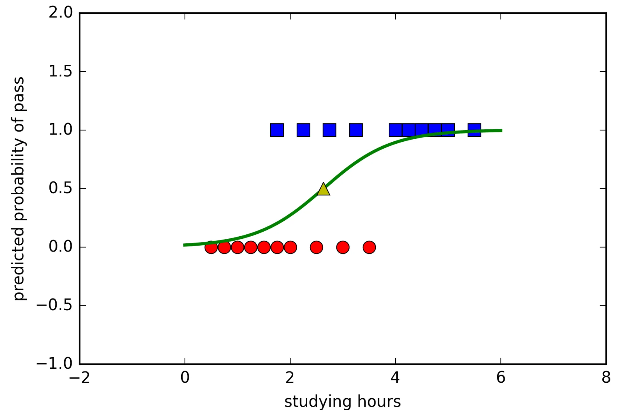
Binary logistic regression is a widely used classification technique that aims to predict the probability of an outcome belonging to one of two classes, usually coded as 0 and 1. Unlike linear regression, where the response variable is continuous, binary logistic regression is designed for binary outcomes. It has significant applications across various domains, including medical diagnostics, risk assessment, and marketing analytics. However, a frequently asked question in statistical modeling is why binary logistic regression does not incorporate a weight matrix like some other types of regression models. This absence is rooted in the nature of logistic regression’s optimization method, its probabilistic interpretation, and the simplicity of working directly with estimated coefficients.
Understanding the Core of Binary Logistic Regression
Binary logistic regression models the relationship between the independent variables (features) and a binary dependent variable. In this model, the probability of the binary outcome is modeled using the logistic (or sigmoid) function, which restricts the output to values between 0 and 1. Mathematically, the model is structured as:
P(Y=1∣X)=11+e−(β0+β1X1+β2X2+⋯+βnXn)P(Y = 1 | X) = \frac{1}{1 + e^{-(\beta_0 + \beta_1X_1 + \beta_2X_2 + \dots + \beta_nX_n)}}P(Y=1∣X)=1+e−(β0+β1X1+β2X2+⋯+βnXn)1
where:
- P(Y=1∣X)P(Y = 1 | X)P(Y=1∣X) is the probability that the output YYY is 1 given the input features XXX,
- β0\beta_0β0 is the intercept term,
- β1,β2,…,βn\beta_1, \beta_2, \dots, \beta_nβ1,β2,…,βn are the coefficients associated with each feature.
The objective of logistic regression is to find the best-fit coefficients β\betaβ that maximize the likelihood of the observed data. The estimation of these coefficients occurs through maximum likelihood estimation (MLE), rather than ordinary least squares (OLS) used in linear regression. This distinction is crucial for understanding the absence of a weight matrix.
Weight Matrices in Regression Models: An Overview
In the context of linear regression, a weight matrix (often referred to as a “weight vector” when considering individual weights for each observation) can be used to emphasize or deemphasize specific observations. In weighted least squares (WLS), each observation in the dataset is multiplied by a weight, allowing the model to focus more heavily on certain data points, often those with lower variance or greater reliability. The weight matrix enables weighted linear regression models to better accommodate heteroscedasticity, where the variability of the dependent variable changes across levels of the independent variables.
However, logistic regression fundamentally differs from linear regression in that it operates within a probabilistic framework where the outcome is categorical. The target in logistic regression is not a continuous variable that can assume any real value but rather a probability of belonging to a specific class. This distinction leads to the absence of a weight matrix in binary logistic regression.
The Role of Maximum Likelihood in Logistic Regression
The coefficients in binary logistic regression are estimated through maximum likelihood estimation (MLE), a method that seeks to maximize the probability of the observed data given the model parameters. MLE differs from OLS because it does not minimize residuals directly; instead, it finds parameters that make the observed outcomes as probable as possible.
In MLE, the probability function is derived from the logistic model, resulting in a log-likelihood function that can be maximized with respect to the parameters. The maximization of the likelihood function inherently considers all observations without the need for a weight matrix. Each observation contributes to the likelihood based on its probability of occurrence under the given parameters, making the addition of a weight matrix redundant in most standard applications.
If one were to introduce a weight matrix into MLE for logistic regression, it could disrupt the probabilistic balance and introduce bias, leading to misleading results. MLE ensures that the estimation is unbiased across all observations, adhering to the assumption that each observation independently and equally represents the underlying probability distribution.
The Interpretation of Coefficients in Logistic Regression
In linear regression, coefficients have an intuitive interpretation: they represent the average change in the dependent variable for a one-unit change in the predictor, holding all else constant. However, in logistic regression, coefficients have a different meaning. They represent the change in the log-odds of the outcome for a one-unit change in the predictor.
Logistic regression coefficients describe the relationship between each predictor and the log-odds of the binary outcome. Adding weights to observations in this context would alter these log-odds in a way that could make the interpretation of coefficients problematic, as the weighting would bias the log-odds toward certain observations. Since the goal in logistic regression is to maximize the likelihood of observing the actual binary outcomes, weighting would complicate this objective without offering a straightforward advantage.
Table: Comparison of Linear and Logistic Regression Features
| Feature | Linear Regression | Binary Logistic Regression |
|---|---|---|
| Target Variable | Continuous | Binary (0 or 1) |
| Estimation Method | Ordinary Least Squares (OLS) | Maximum Likelihood Estimation (MLE) |
| Interpretation of Coefficients | Direct change in dependent variable | Change in log-odds of outcome |
| Use of Weight Matrix | Often used in Weighted Least Squares | Not typically included |
| Objective | Minimize residual sum of squares | Maximize likelihood of observed outcomes |
Probabilistic Interpretation and the Sigmoid Function
The logistic regression model uses the sigmoid function to transform the linear combination of the features and coefficients into a probability value between 0 and 1. The sigmoid function’s steep slope around 0.5 allows logistic regression to handle probabilities effectively, which would be distorted by a weight matrix.

Adding a weight matrix in this probabilistic context is not necessary because the probability model inherently assigns varying levels of influence to different observations based on their fit to the predicted log-odds. The log-likelihood function for logistic regression already accounts for how well each observation fits the model. This function does not assume equal variability across the observations but instead focuses on the alignment of observed binary outcomes with the predicted probabilities.
Practical Implications of No Weight Matrix
While binary logistic regression does not natively include a weight matrix, there are methods for adjusting the model in specialized situations. For example, if one has imbalanced classes or wants to handle specific types of data weighting (e.g., in cases of survey data where each observation has an associated probability weight), the solution typically involves alternative forms of logistic regression, such as penalized logistic regression or Bayesian approaches. These methods adjust for certain data characteristics without introducing a weight matrix that might distort the maximum likelihood estimation.
Addressing Class Imbalance Without a Weight Matrix
In scenarios with severe class imbalance, logistic regression can struggle because it might be biased toward the majority class. A common workaround is to use resampling techniques, such as oversampling the minority class or undersampling the majority class, instead of applying a weight matrix. Another alternative is to apply a threshold adjustment, setting a different decision boundary for classification based on desired sensitivity or specificity. Such techniques are preferred in logistic regression for dealing with class imbalance, as they maintain the model’s probabilistic integrity without resorting to weighted observations.
The absence of a weight matrix in binary logistic regression is a result of the model’s reliance on maximum likelihood estimation, probabilistic interpretation of coefficients, and the sigmoid function’s properties. Logistic regression’s design centers on maximizing the likelihood of observed binary outcomes, making a weight matrix unnecessary and potentially disruptive to the model’s interpretation.
In logistic regression, each observation contributes to the likelihood function without the need for explicit weighting, as the optimization inherently balances the influence of each data point. This method aligns with the logistic model’s purpose: to provide a clear, interpretable probability of class membership without skewed influence from certain observations. Therefore, logistic regression remains effective and interpretable without a weight matrix, emphasizing its role as a foundational tool in binary classification.


